1.4.1. CURVE GEOMETRY
NURBS (non-uniform rational B-splines) are mathematical representations that can accurately model any shape from a simple 2D line, circle, arc, or box to the most complex 3D free-form organic surface or solid. Because of their flexibility and accuracy, NURBS models can be used in any process from illustration and animation to manufacturing.
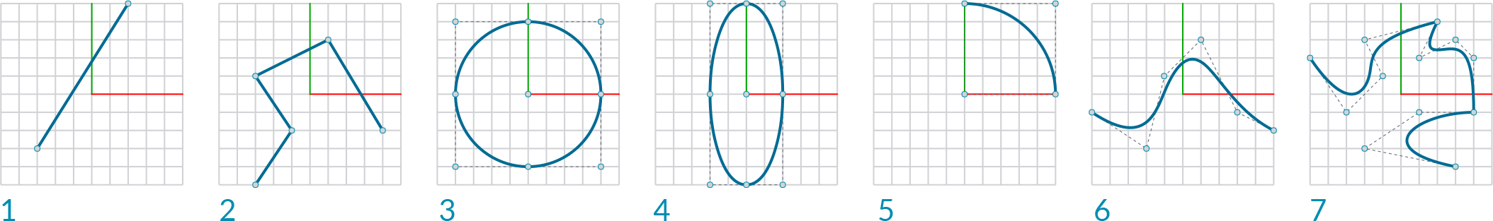
Since curves are geometric objects, they possess a number of properties or characteristics which can be used to describe or analyze them. For example, every curve has a starting coordinate and every curve has an ending coordinate. When the distance between these two coordinates is zero, the curve is closed. Also, every curve has a number of control-points, if all these points are located in the same plane, the curve as a whole is planar. Some properties apply to the curve as a whole, while others only apply to specific points on the curve. For example, planarity is a global property while tangent vectors are a local property. Also, some properties only apply to some curve types. So far we’ve discussed some of Grasshopper’s Primitive Curve Components such as: lines, circles, ellipses, and arcs.
- Line
- Polyline
- Circle
- Ellipse
- Arc
- NURBS Curve
- Polycurve
- End Point
- Edit Point
- Control Point
1.4.1.1. NURBS CURVES
Degree: The degree is a positive whole number. This number is usually 1, 2, 3 or 5, but can be any positive whole number. The degree of the curve determines the range of influence the control points have on a curve; where the higher the degree, the larger the range. NURBS lines and polylines are usually degree 1, NURBS circles are degree 2, and most free-form curves are degree 3 or 5.
Control Points: The control points are a list of at least degree+1 points. One of the easiest ways to change the shape of a NURBS curve is to move its control points.
Weight: Control points have an associated number called a weight . Weights are usually positive numbers. When a curve’s control points all have the same weight (usually 1), the curve is called non-rational, otherwise the curve is called rational. Most NURBS curves are non-rational. A few NURBS curves, such as circles and ellipses, are always rational.
Knots: Knots are a list of (degree+N-1) numbers, where N is the number of control points.
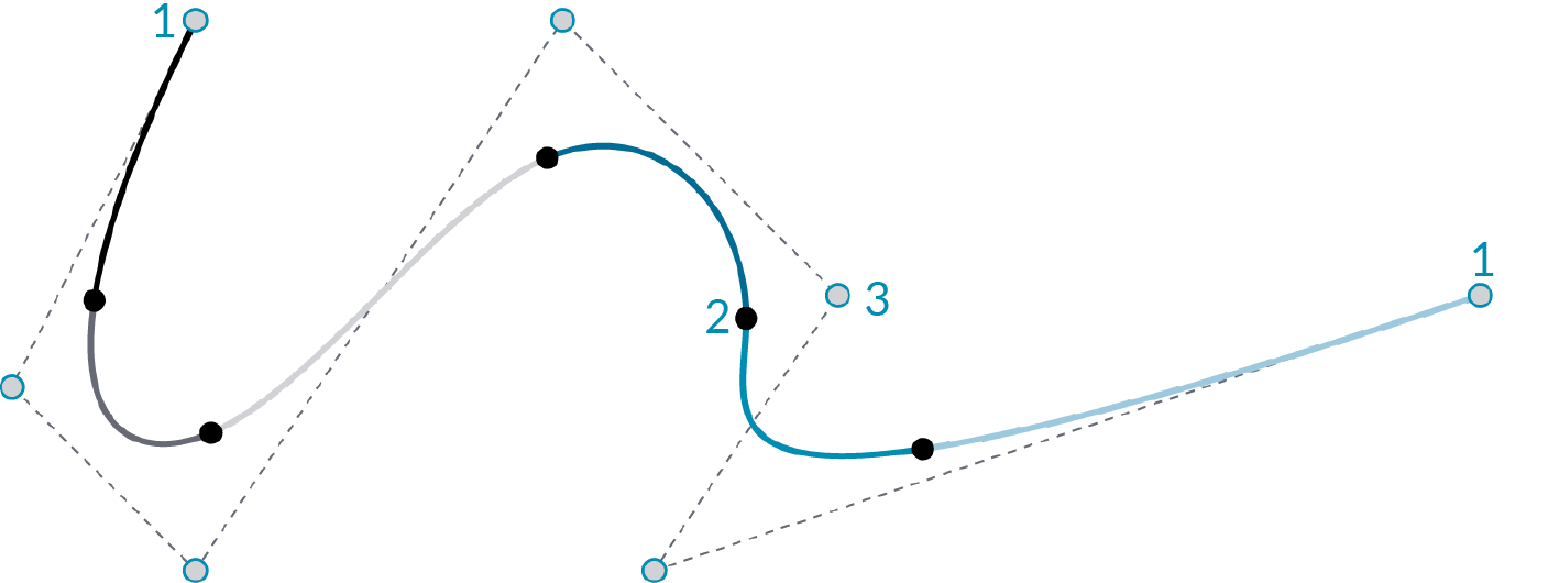
Edit Points: Points on the curve evaluated at knot averages. Edit points are like control points except they are always located on the curve and moving one edit point generally changes the shape of the entire curve (moving one control point only changes the shape of the curve locally). Edit points are useful when you need a point on the interior of a curve to pass exactly through a certain location.
NURBS curve knots as a result of varying degree:
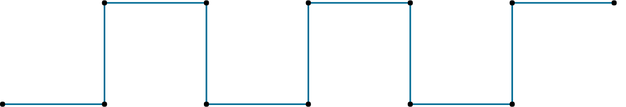
A D1 NURBS curve behaves the same as a polyline. A D1 curve has a knot for every control point.
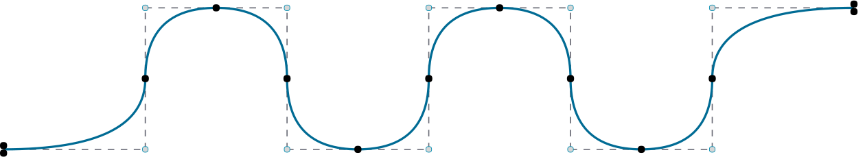
D2 NURBS curves are typically only used to approximate arcs and circles. The spline intersects with the control polygon halfway each segment.
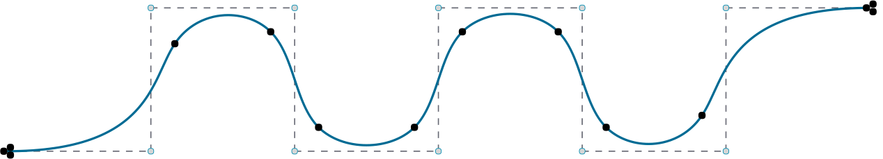
D3 is the most common type of NURBS curve and is the default in Rhino. You are probably very familiar with the visual progression of the spline, even though the knots appear to be in odd locations.
1.4.1.2. GRASSHOPPER SPLINE COMPONENTS
Example files that accompany this section: Download
Grasshopper has a set of tools to express Rhino’s more advanced curve types like nurbs curves and poly curves. These tools can be found in the Curve/Splines tab.
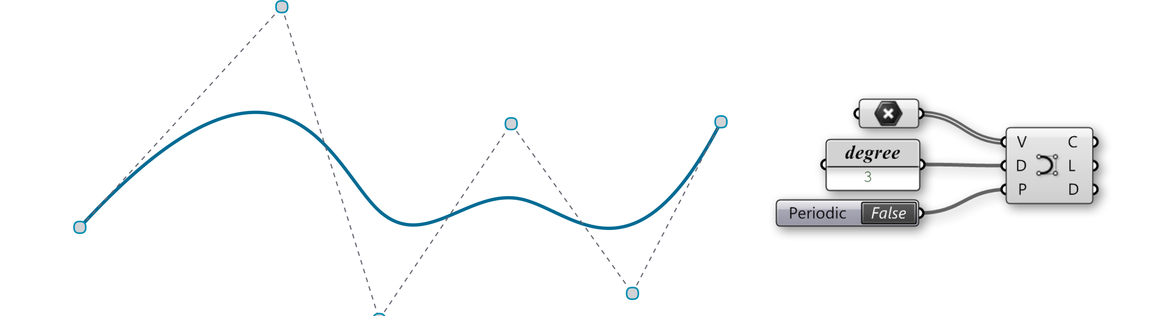
Nurbs Curve (Curve/Spline/Nurbs curve): The Nurbs Curve component constructs a NURBS curve from control points. The V input defines these points, which can be described implicitly by selecting points from within the Rhino scene, or by inheriting volatile data from other components. The Nurbs Curve-D input sets the degree of the curve.
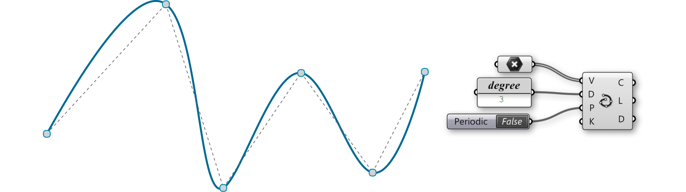
Interpolate Curve (Curve/Spline/Interpolate): Interpolated curves behave slightly differently than NURBS curves. The V-input is for the component is similar to the NURBS component, in that it asks for a specific set of points to create the curve. However, with the Interpolated Curve method, the resultant curve will actually pass through these points, regardless of the curve degree. In the NURBS curve component, we could only achieve this when the curve degree was set to one. Also, like the NURBS curve component, the D input defines the degree of the resultant curve. However, with this method, it only takes odd numbered values for the degree input. Again, the P-input determines if the curve is Periodic. You will begin to see a bit of a pattern in the outputs for many of the curve components, in that, the C, L, and D outputs generally specify the resultant curve, the length, and the curve domain respectively.
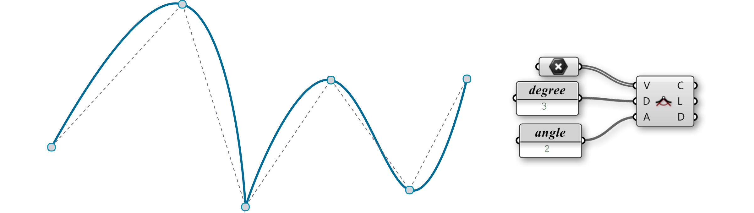
Kinky Curve (Curve/Spline/Kinky Curve): The kinky curve component allows you the ability to control a specific angle threshold, A, where the curve will transition from a kinked line, to a smooth, interpolated curve. It should be noted that the A-input requires an input in radians.
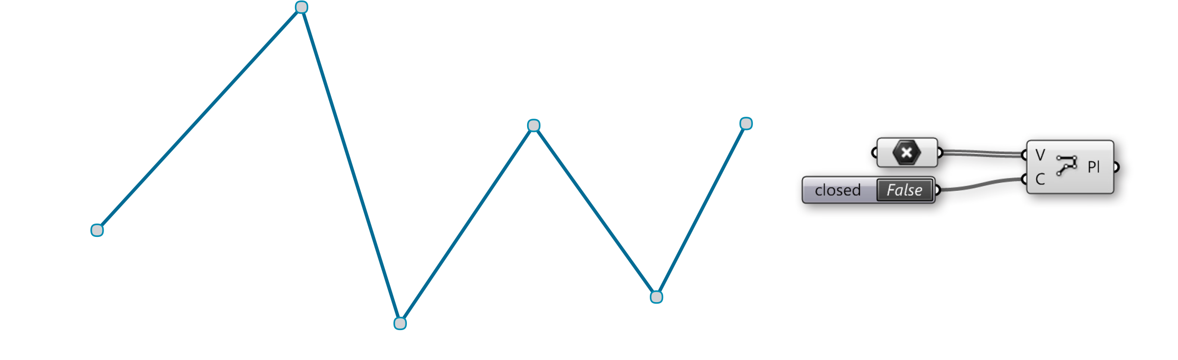
Polyline (Curve/Spline/Polyline): A polyline is a collection of line segments connecting two or more points, the resultant line will always pass through its control points; similar to an Interpolated Curve. Like the curve types mentioned above, the V-input of the Polyline component specifies a set of points that will define the boundaries of each line segment that make up the polyline. The C-input of the component defines whether or not the polyline is an open or closed curve. If the first point location does not coincide with the last point location, a line segment will be created to close the loop. The output for the Polyline component is different than that of the previous examples, in that the only resultant is the curve itself.