1.5.4. Working with Data Trees
Example files that accompany this section: http://grasshopperprimer.com/appendix/A-2/1_gh-files.html
In this example, we will use some of Grasshopper’s tools for manipulating data trees to retreive, reorganize, and interpolate the desired points contained in a data tree and create a lattice of intersecting fins.
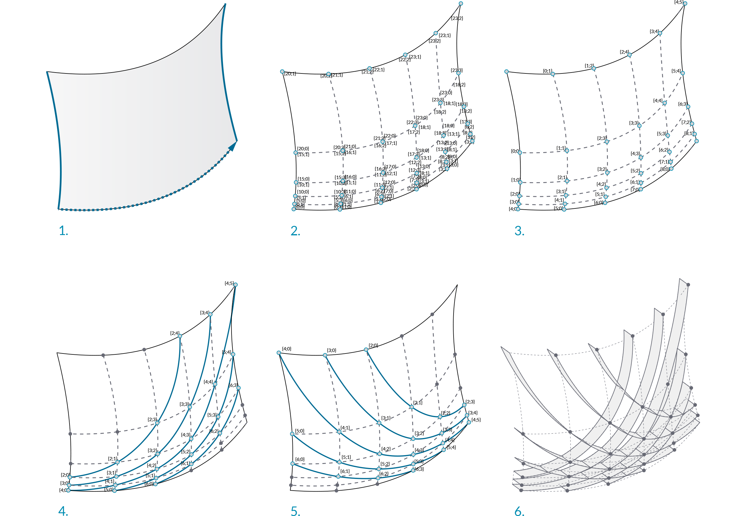
- Sweep with two rails to create a NURBS surface.
- Divide the surface into variable sized segments, extract vertices. Data comprised of one list with four items in each segment.
- Flip the matrix to change the data structure. Data comprised of four lists, each containing a single corner point of each segment.
- Explode the tree to connect corner points and draw diagonal lines across each segement.
- Prune the tree to cull branches containing insufficient points to construct a degree 3 NURBS curve and interpolate points.
- Extrude the curves to create intersecting fins.
| 01. | Start a new definition, type Ctrl+N (in Grasshopper) | |
| 02. | Params/Geometry/Curve – Drag and drop three curve parameters onto the canvas |  |
| 03. | Surface/Freeform/Sweep2 – Drag a Sweep2 component onto the canvas | 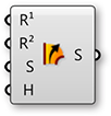 |
| 04. | Right-click the first Curve parameter and select “Set one curve.” Select the first rail curve in the Rhino viewport | |
| 05. | Right-click the second Curve parameter and select “Set one curve.” Select the second rail curve in the Rhino viewport | |
| 06. | Right-click the third Curve parameter and select “Set one curve.” Select the section curve in the Rhino viewport | |
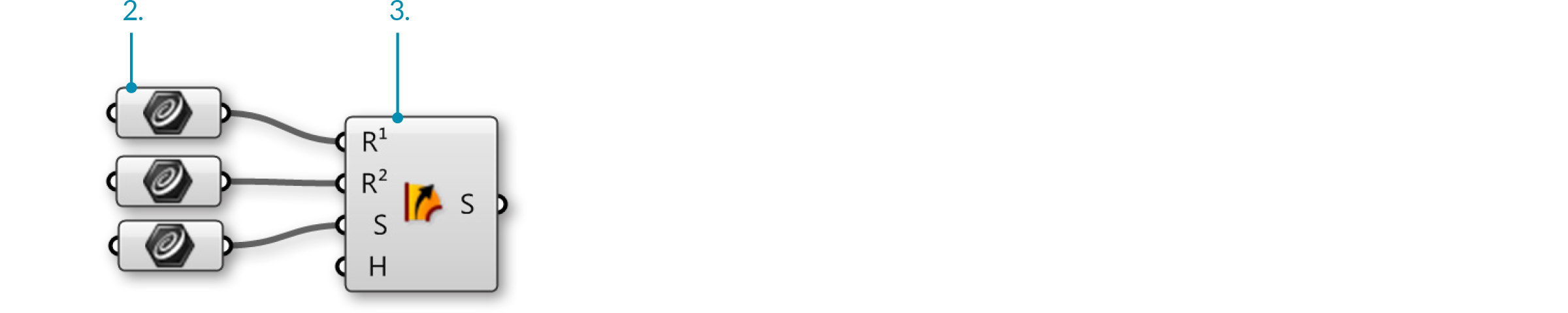
| 07. | Connect the outputs of the Curve parameters to the Rail 1 (R1), Rail 2 (R2), and Sections (S) inputs of the Sweep2 respectively |
We have just created a NURBS surface
| 08. | Params/Geometry/Surface – drag a Surface parameter to the canvas |  |
| 09. | Connect the Brep (S) output of the Sweep2 component to the input of the Surface parameter | |
| 10. | Right-click the Surface parameter and select “Reparameterize”. In this step, we re-mapped the u and v domains of the surface between 0 and 1. This will make future operations possible. |
 |
| 11. | Maths/Domain/Divide Domain2 – drag and drop a Divide Domain2 component onto the canvas |  |
| 12. | Params/Input/Number Slider – drag two Number Sliders onto the canvas | |
| 13. | Double click the first Number Sliders and set the following:
Lower Limit: 1 Upper Limit: 40 Value: 20 |
|
| 14. | Set the same values on the second Number Sliders | |
| 15. | Connect the output of the reparameterized Surface parameter to the Domain (I) input of the Divide Domain2 component | |
| 16. | Connect the first Number Sliders to the U Count (U) input of the Divide Domain2 component | |
| 17. | Connect the second Number Sliders to the V Count (V) input of the Divide Domain2 component | |
| 18. | Surface/Util/Isotrim – Drag and drop the Isotrim component onto the canvas |  |
| 19. | Connect the Segments (S) output of the Divide Domain2 component to the Domain (D) input of the Isotrim component | |
| 20. | Connect the output of the Surface parameter to the Surface (S) input of the Isotrim component |
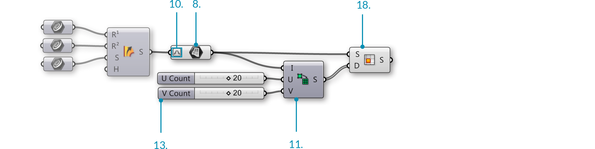
We have now divided out surface into smaller, equally sized, surfaces. Adjust the U and V Count sliders to change the number of divisions. Lets add a Graph Mapper to give the segments variable size.
| 21. | Maths/Domain/Deconstruct Domain2 – Drag a Deconstruct Domain2 component onto the canvas | 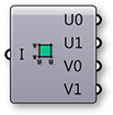 |
| 22. | Maths/Domain/Construct Domain2 – Drag a Construct Domain2 component to the canvas | 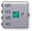 |
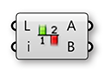
| 23. | Params/Input/Graph Mapper – Drag a Graph Mapper to the canvas | 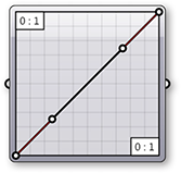 |
| 24. | Sets/List/List Length – Drag a List Length component to the canvas |  |
| 25. | Sets/Tree/Merge – Drag a Merge component to the canvas | 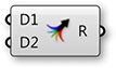 |
| 26. | Sets/List/Split List – Drag a Split List component to the canvas The Merge and Split components are used here so that the same Graph Mapper could be used for both the U min and U max values. |
 |
| 27. | Connect the U min (U0) and U max (U1) outputs of the Deconstruct Domain2 component to the Data 1 (D1) and Data 2 (D2) inputs of the Merge component | |
| 28. | Connect the Result (R) output of the Merge component to the input of the Graph Mapper | |
| 29. | Right-click the Graph Mapper and select “Bezier” under “Graph Types” | |
| 30. | Connect a second wire from the U max (U1) output of the Deconstruct Domain2 component to the List (L) input of the List Length component | |
| 31. | Connect the Graph Mapper output to the List (L) input of the Split List | |
| 32. | Connect the Length (L) output of the List Length component to the Index (i) input of the Split List component | |
| 33. | Connect the List A (A) output of the Split List component to the U min (U0) input of the Construct Domain2 component | |
| 34. | Connect the List B (B) output of the Split List component to the U max (U1) input of the Construct Domain2 component | |
| 35. | Connect the V min (V0) output of the Deconstruct Domain2 component to the V min (V1) input of the Construct Domain2 component | |
| 36. | Connect the V max (V1) output of the Deconstruct Domain2 component to the V max (V1) input of the Construct Domain2 component | |
| 37. | Connect the 2D Domain (I2) output of the Construct Domain2 component to the Domain (D) input of the Isotrim component, replacing the existing connection |
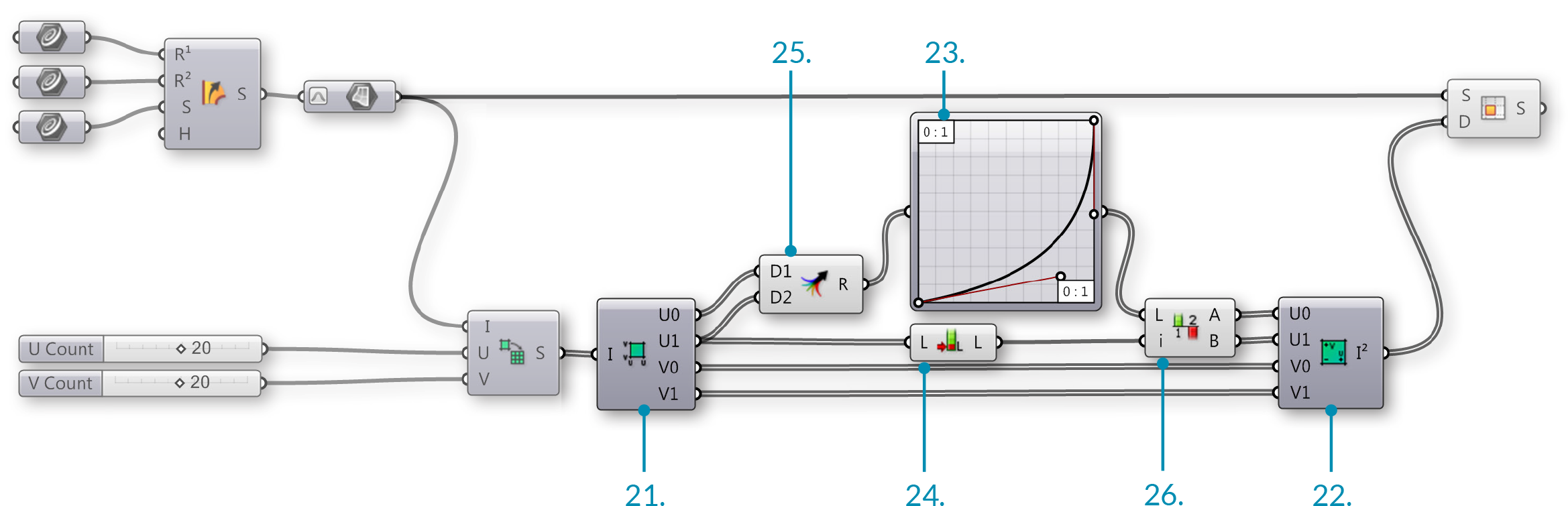
We have just deconstructed the domains of each surface segment, remapped the U values using a Graph Mapper, and reconstructed the domains. Adjust the grips of the Graph Mapper to change the distribution of the surface segments. Let’s use Data Trees to manipulate the surface divisions.
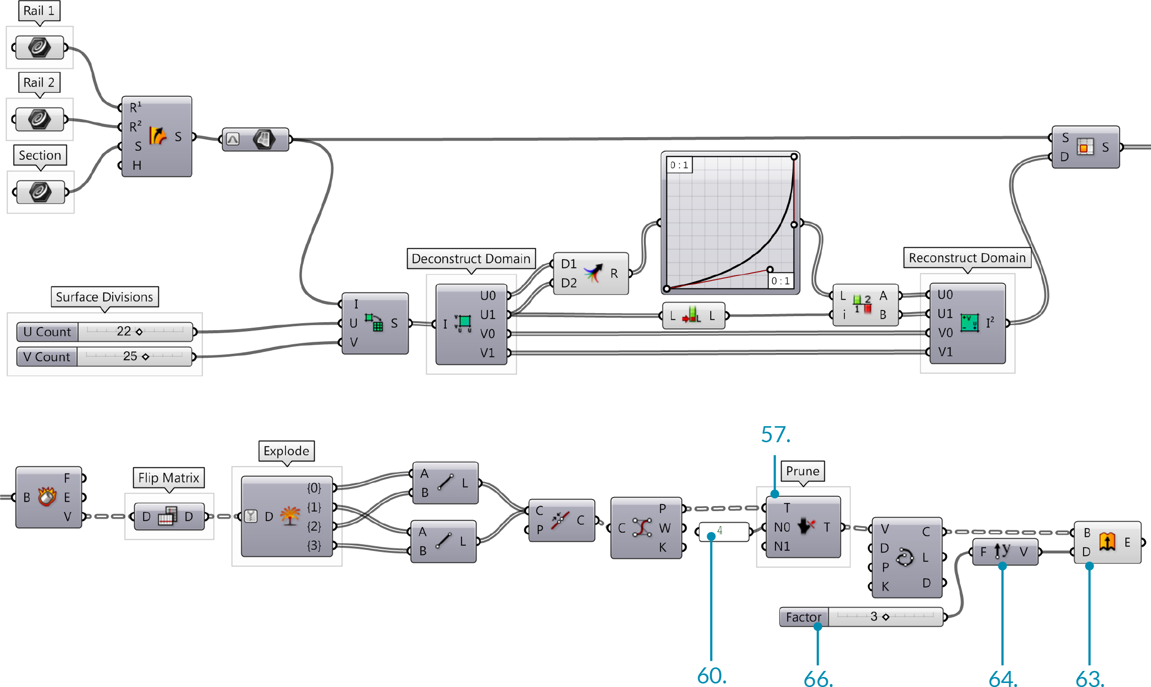
| 38. | Surface/Analysis/Deconstruct Brep – Drag the Deconstruct Brep component onto the canvas |  |
| 39. | Sets/Tree/Flip Matrix – Drag the Flip Matrix component to the canvas |  |
| 40. | Sets/Tree/Explode Tree – Drag the Explode Tree component to the canvas |  |
| 41. | Connect the Surface (S) output of the Isotrim component to the Brep (B) input of the Deconstruct Brep component The Deconstruct Brep component deconstructs a Brep into Faces, Edges, and Vertices. This is helpful if you want to operate on a specific constituent of the surface. |
|
| 42. | Connect the Vertices (V) output of the Deconstruct Brep component to the Data (D) input of the Flip Matrix component We just changed the Data tree structure from one list of four vertices that define each surface, to four lists, each containing one vertex of each surface. |
|
| 43. | Connect the Data (D) output of the Flip Matrix component to the Data (D) input of the Explode Tree component | |
| 44. | Right-click the Explode Tree component and select “Match Outputs” | |
| 45. | Right-click the Data (D) input of the Explode Tree component and select simplify |
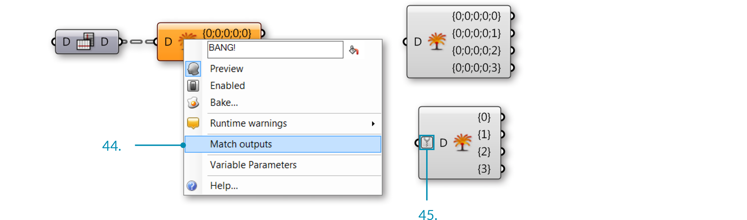
Each output of the Explode Tree component contains a list of one vertex of each surface. In other words, one list with all the top right corners, one list with all the bottom right corners, one list of top left corners, and one list of bottom left corners.
| 46. | Curve/Primitive/Line – Drag and drop two Line components onto the canvas |  |
| 47. | Connect the Branch 0 {0} output of the Explode Tree component to the Start Point (A) input of the first Line component | |
| 48. | Connect the Branch 1 {1} output of the Explode Tree component to the Start Point (A) input of the second Line component | |
| 49. | Connect the Branch 2 {2} output of the Explode Tree component to the End Point (B) input of the first Line component | |
| 50. | Connect the Branch 3 {3} output of the Explode Tree component to the End Point (B) input of the second Line component |

We have now connected the corner points of each surface diagonally with lines.
| 51. | Curve/Util/Join Curves – Drag and drop the Join Curves component to the canvas |  |
| 52. | Curve/Analysis/Control Points – Drag a Control Points component onto the canvas | 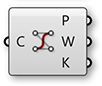 |
| 53. | Curve/Spline/Interpolate – Drag and drop the Interpolate component onto the canvas |  |
| 54. | Connect the Line (L) outputs of each Line component to the Curves (C) input of the Join Curves component Hold down the Shift key to connect multiple wires to a single input |
|
| 55. | Connect the Curves (C) output of the Join Curves component to the Curve (C) input of the Control Points component | |
| 56. | Connect the Points (P) output of the Control Points component to the Vertices (V) input of the Interpolate component |
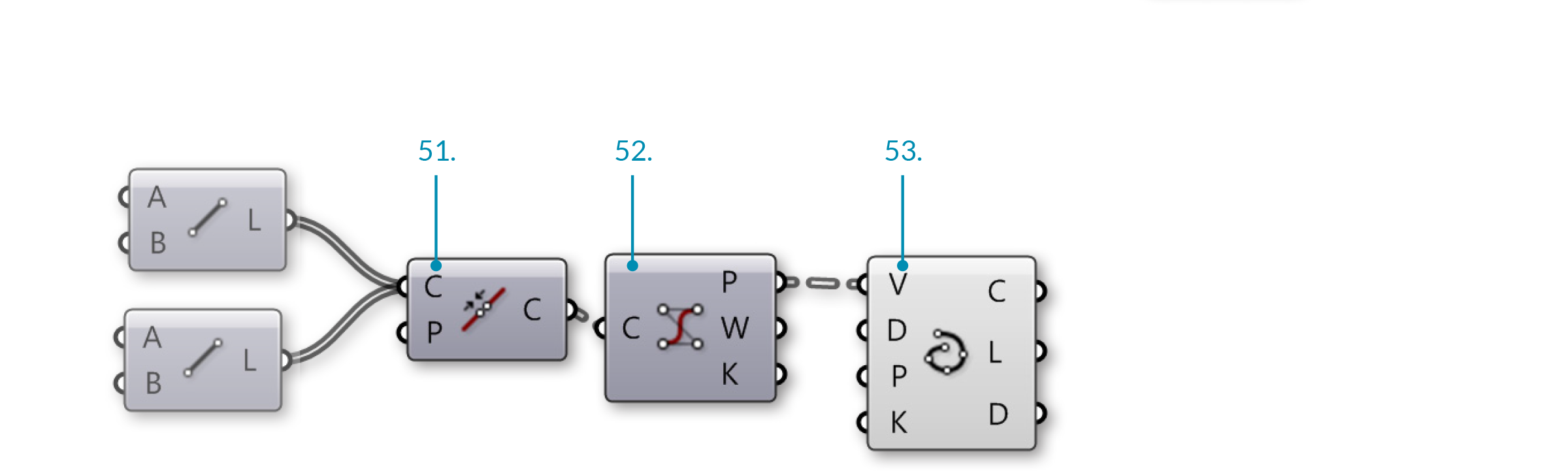
We have now joined our lines into polylines and reconstructed them as NURBS curves by interpolating their control points. In the Rhino viewport, you might notice that the shorter curves are still straight lines. This is because you cannot make a degree three NURBS curve with fewer than four control points. Let’s manipulate the data tree to eliminate lists of control points with less than four items.
| 57. | Sets/Tree/Prune Tree – Drag and drop the Prune Tree component onto the canvas |  |
| 58. | Params/Input/Panel – Drag a Panel onto the canvas | |
| 59. | Connect the Points (P) output of the Control Points component to the Tree (T) input of the Prune Tree component If you connect one Param Viewer to the Points (P) output of the Control Points component, and another to the Tree (T) output of the Prune Tree component, you can see that the number of branches has been reduced. |
|
| 60. | Double click the Panel and enter 4. |  |
| 61. | Connect the output of the Panel to the Minimum (N0) input of the Prune Tree component | |
| 62. | Connect the Tree (T) output of the Prune Tree component to the Vertices (V) input of the Interpolate component | |
| 63. | Surface/Freeform/Extrude – Drag and drop the Extrude component onto the canvas |  |
| 64. | Vector/Vector/Unit Y – Drag a Unit Y component onto the canvas You may need to use a Unit X vector, depending on the orientation of your referenced geometry in Rhino |
 |
| 65. | Params/Input/Number Slider – Drag a Number Slider onto the canvas | |
| 66. | Double click the Number Slider and set the following:
Lower Limit: 1 Upper Limit: 5 Value: 3 |
|
| 67. | Connect the Curve (C) output of the Interpolate component to the Base (B) input of the Extrude component | |
| 68. | Connect the Number Slider output to the Factor (F) input of the Unit Y component | |
| 69. | Connect the Unit Vector (V) output of the Unit Y component to the Direction (D) input of the Extrude component |
You should now see a diagonal grid of strips or fins in the Rhino Viewport. Adjust the Factor slider to chnage the depth of the fins